写在前面 昨天写了基于感知机的鸢尾花分类,今天下午要考《大数据技术原理》,本来是整个白天的课程设计,因为考试少了一下午。之前看书复习了一波,但记忆是需要反复锤炼的,所以要抓紧写完这个传播算法,抽出时间再去复习会。2021.11.30/2021.12.1/2021.12.2
以人事招聘为例的误差反向传播算法 实验目的 理解多层神经网络的结构和原理,掌握反向传播算法对神经元的训练过程,了解反向传播公式。通过构建 BP 网络实例,熟悉前馈网络的原理及结构。
背景知识 误差反向传播算法即 BP 算法,是一种适合于多层神经网络的学习算法。其建立在梯度下降方法的基础之上,主要由激励传播和权重更新两个环节组成,经过反复迭代更新、修正权值从而输出预期的结果。BP 算法整体上可以分成正向传播和反向传播,原理如下:正向传播过程:信息经过输入层到达隐含层,再经过多个隐含层的处理后到达输出层。反向传播过程:比较输出结果和正确结果,将误差作为一个目标函数进行反向传播:对每一层依次求对权值的偏导数,构成目标函数对权值的梯度,网络权重再依次完成更新调整。依此往复、直到输出达到目标值完成训练。该算法可以总结为:利用输出误差推算前一层的误差,再用推算误差算出更前一层的误差,直到计算出所有层的误差估计。1986 年,Hinton 在论文《Learning Representations by Back-propagating Errors》中首次系统地描述了如何利用 BP 算法来训练神经网络。从此,BP 算法开始占据有监督神经网络算法的核心地位。它是迄今最成功的神经网络学习算法之一,现实任务中使用神经网络时,大多是在使用 BP 算法进行训练。
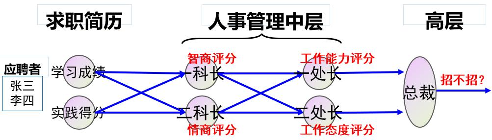
为了说明 BP 算法的过程,本实验使用一个公司招聘的例子:假设有一个公司,其人员招聘由 5个人组成的人事管理部门负责,如下图所示:
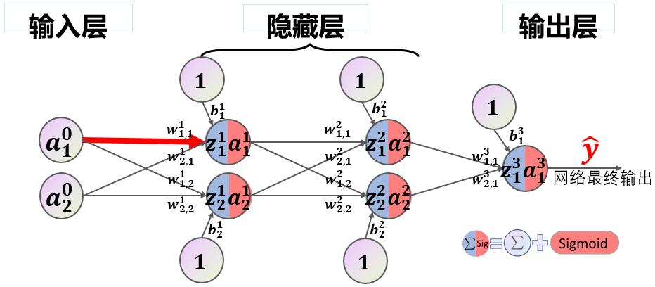
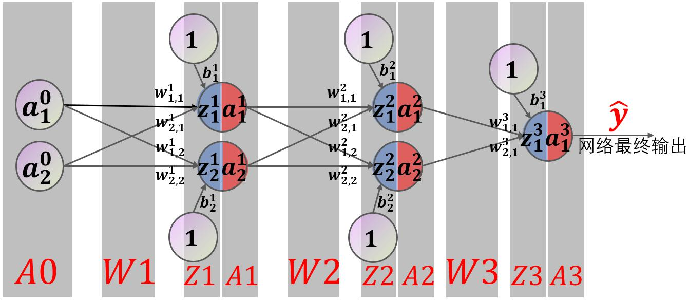
其中张三、李四等人是应聘者,他们向该部门投递简历,简历包括两类数据:学习成绩和社会实践得分,人事部门有三个层级,一科长根据应聘者的学习成绩和实践得分评估其智商,二科长根据同样的资料评估其情商;一处长根据两个科长提供的智商、情商评分,评估应聘者的工作能力,二处长评估工作态度;最后由总裁汇总两位处长的意见,得出最终结论,即是否招收该应聘者。该模型等价于一个形状为(2,2,2,1)的前馈神经网络,输入层、隐藏层 1、隐藏层 2、输出层各自包含 2、2、2、1 个节点,如下图所示。
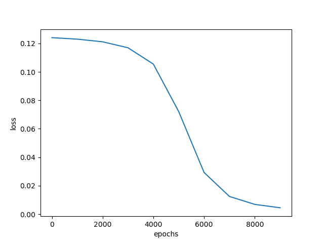
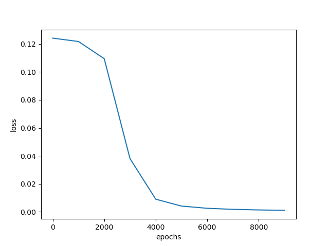
示例代码 1 2 3 4 5 6 7 8 9 10 11 12 13 14 15 16 17 18 19 20 21 22 23 24 25 26 27 28 29 30 31 32 33 34 35 36 37 38 39 40 41 42 43 44 45 46 47 48 49 50 51 52 53 54 55 56 57 58 59 60 61 62 63 64 65 66 67 68 69 70 71 72 73 74 75 76 77 78 79 80 81 82 83 84 85 86 87 88 89 90 91 92 93 94 95 96 97 98 99 100 101 102 103 104 105 106 107 108 109 110 111 112 113 114 115 116 117 118 119 120 121 122 123 124 125 126 127 128 129 130 131 132 133 134 135 136 137 138 139 140 141 142 143 144 145 146 147 148 149 150 151 152 153 154 155 156 157 158 159 160 import numpy as npimport matplotlib.pyplot as plt1 ,0.1 ]])1 ]])0.8 ,0.2 ],0.2 ,0.8 ]])0.5 ,0.0 ],0.5 ,1.0 ]])0.5 ],0.5 ]])1 ,0.3 ]])0.1 ,-0.1 ]])0.6 ]])0.1 10000 1000 1 def sigmoid (x ):return 1 /(1 +np.exp(-x))def dsigmoid (x ):return x*(1 -x)def update ():global batch_X,batch_T,W1,W2,W3,lr,b1,b2,b30 ]sum (delta_Z3, axis=0 ) / batch_X.shape[0 ]0 ]sum (delta_Z2, axis=0 ) / batch_X.shape[0 ]0 ]sum (delta_Z1, axis=0 ) / batch_X.shape[0 ]0 ] // batch_sizefor idx_epoch in range (epochs):for idx_batch in range (max_batch):1 )*batch_size, :]1 )*batch_size, :]if idx_epoch % report == 0 :'A3:' ,A3)'epochs:' ,idx_epoch,'loss:' ,np.mean(np.square(T - A3) / 2 ))2 ))range (0 ,epochs,report),loss)'epochs' )'loss' )'output:' )def predict (x ):if x>=0.5 :return 1 else :return 0 'predict:' )for i in map (predict,A3):
实验内容 请回答下列问题:
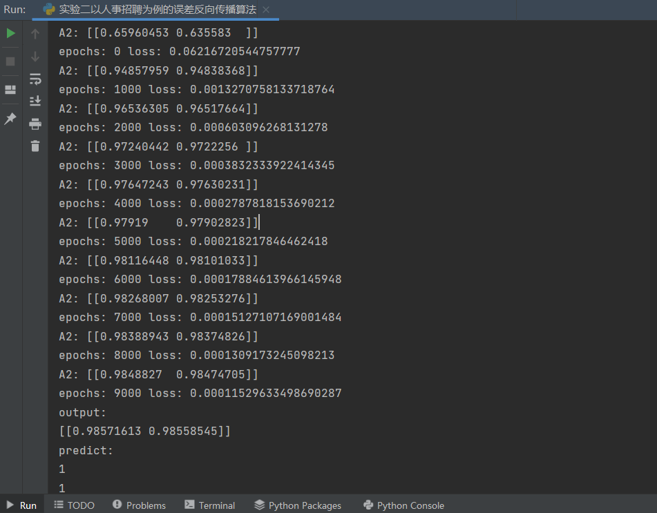
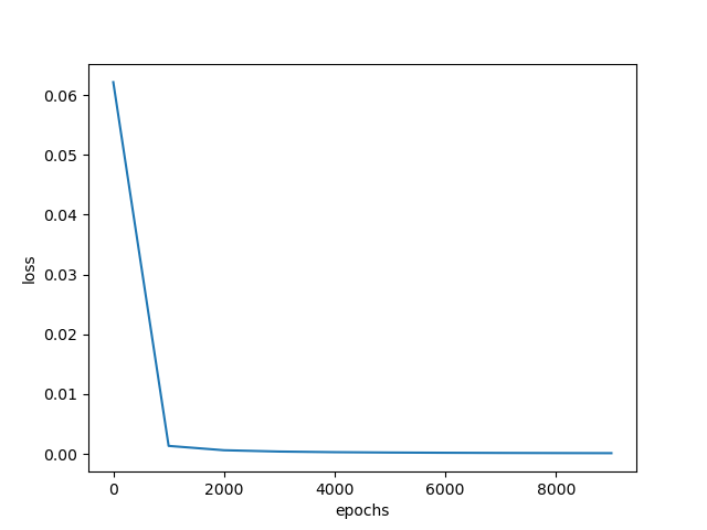
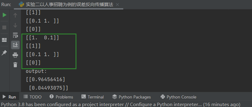
第一题 1. 如果去掉总裁这一层,相应张三的样本修改为(1.0,0.1,1.0,1.0),分别对应张三的学习成绩、张三的实践成绩、张三的工作能力真值、张三的工作态度真值,代码应该如何修改?
要修改的代码:
更改的:
1 2 3 4 5 6 7 8 9 10 11 12 80. delta_A2 = delta_Z3.dot(batch_T - A2)127. print('A2:' ,A2)128. print('epochs:' ,idx_epoch,'loss:' ,np.mean(np.square(T - A2) / 2 ))130. loss.append(np.mean(np.square(T - A2) / 2 ))145. print(A3)159. for i in map (predict,A2.T):
删除的:
1 2 3 4 5 6 7 8 9 10 11 12 13 14 15 16 17 18 19 20 21 22 23 24 25 27. W3 = np.array([[0.5 ],28. [0.5 ]])37. b3 = np.array([[-0.6 ]])68. Z3=(np.dot(A2,W3) + b3)69. A3 = sigmoid(Z3)72. delta_A3 = (batch_T - A3)73. delta_Z3 = delta_A3 * dsigmoid(A3)76. delta_W3 = A2.T.dot(delta_Z3) / batch_X.shape[0 ]77. delta_B3 = np.sum (delta_Z3, axis=0 ) / batch_X.shape[0 ]96. W3 = W3 + lr *delta_W3101. b3 = b3 + lr * delta_B3125. A3 = sigmoid(np.dot(A2,W3) + b3)143. A3 = sigmoid(np.dot(A2,W3) + b3)
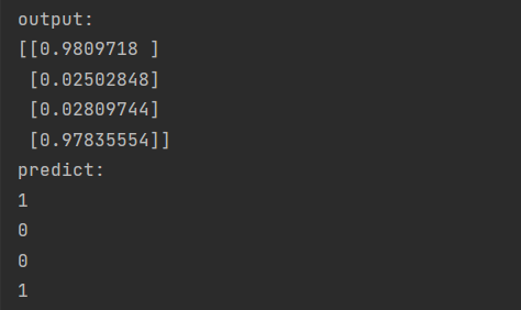
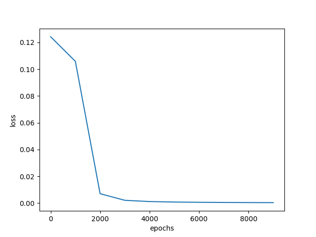
结果:
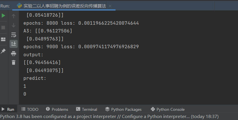
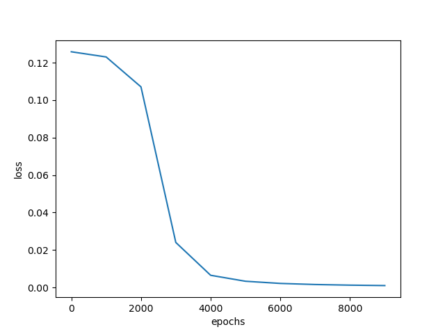
第二题 2..如果增加一个样本,李四(0.1,1.0,0),分别对应李四的学习成绩,李四的实践成绩,李四被招聘可能性的真值,代码应该如何修改?此时是一个样本计算一次偏导、更新一次权值,还是两个样本一起计算一次偏导、更新一次权值?(提示:注意 batch_size 的作用)
修改的代码:
1 2 3 4 5 6 5. X = np.array([[1 ,0.1 ],0.1 ,1 ]])11. T = np.array([[1 ],0 ]])
结果:
此时,我们通过修改代码:
1 2 3 4 5 6 7 8 9 114. for idx_batch in range (max_batch):1 )*batch_size, :]1 )*batch_size, :]
运行程序不难看出:
当batch_size==1时,一个样本计算一次偏导,更新一次权值。
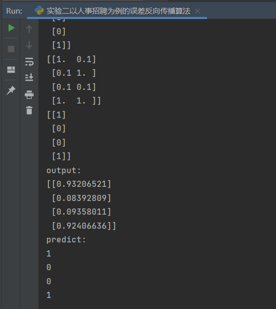
第三题 3.样本为张三[1,0.1,1]、李四[0.1,1,0]、王五[0.1,0.1,0]、赵六[1,1,1],请利用 batch_size 实现教材 279 页提到的“批量梯度下降”、“随机梯度下降”和“小批量梯度下降”,请注意“随机梯度下降”和“小批量梯度下降”要体现随机性。
批量梯度下降 修改代码:
1 2 3 4 5 6 7 8 9 10 11 12 13 4. 1 ,0.1 ],0.1 ,1 ],0.1 ,0.1 ],1 ,1 ]])1 ],0 ],0 ],1 ]])4
此时,四个样本一起计算一次偏导,更新一次权值,进行一次迭代。符合在每一次迭代时 使用所有样本 来进行梯度的更新。
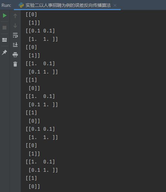
随机梯度下降训练结果:
随机梯度下降 修改代码:
1 2 3 4 5 6 7 8 9 10 1 114. for idx_batch in range (max_batch):0 ,max_batch-1 )1 )*batch_size, :]1 )*batch_size, :]
随机性体现如下:
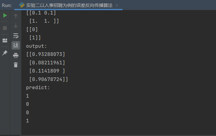
随机批量梯度下降法结果:
小批量梯度下降 在这里,我们设置小批量梯度下降的m为2.
修改代码:
1 2 3 4 5 6 7 8 9 10 11 12 13 2 for idx_batch in range (max_batch):1 ,1.5 ,2 ])0 ,2 )int ((r_nums[r_num]-1 ))*batch_size:(int (r_nums[r_num]))*batch_size]int ((r_nums[r_num]-1 ))*batch_size:(int (r_nums[r_num]))*batch_size]
小批量随机梯度下降结果:
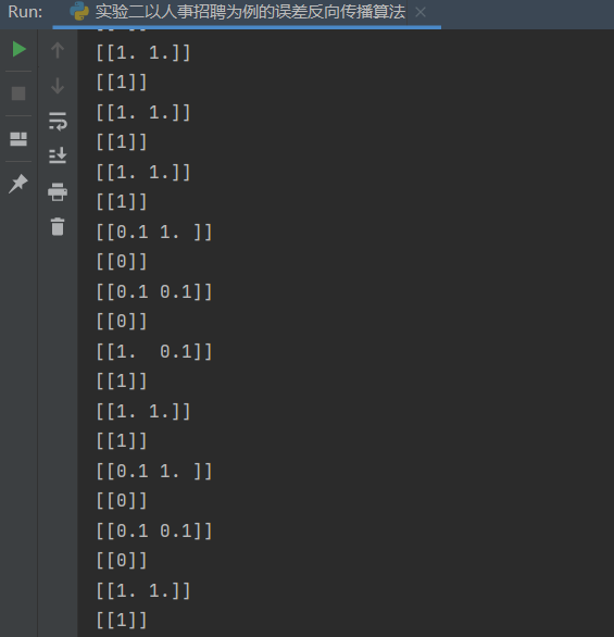
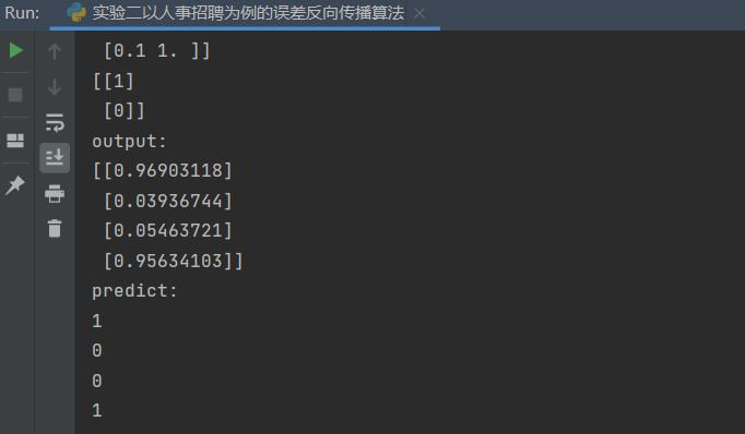
第四题 4.【 选 做 】 本 例 中 输 入 向 量 、 真 值 都 是 行 向 量 , 请 将 它 们 修 改 为 列 向 量 , 如X = np.array([[1,0.1]])改为 X = np.array([[1],[0.1]]),请合理修改其它部分以使程序得到与行向量时相同的结果。
基于第三题小批量随机梯度 下降更改的代码:
1 2 3 4 5 6 7 8 9 10 11 12 13 14 15 16 17 18 19 20 21 22 23 24 25 26 27 28 29 30 31 32 33 34 35 36 37 38 39 40 41 42 43 44 45 46 47 48 49 50 51 52 53 54 55 56 57 58 59 60 61 62 63 64 65 66 67 68 69 70 71 72 73 74 75 76 77 78 79 80 81 82 83 84 85 86 87 88 89 90 91 92 93 94 95 96 97 98 99 100 101 102 103 104 105 106 107 108 109 110 111 112 113 114 115 116 117 118 119 120 121 122 123 124 125 126 127 128 129 130 131 132 133 134 135 136 137 138 139 140 141 142 143 144 145 146 147 148 149 150 151 152 153 154 155 156 157 158 159 160 161 162 163 164 165 166 167 168 169 170 import randomimport numpy as npimport matplotlib.pyplot as plt1 ,0.1 ,0.1 ,1 ],0.1 ,1 ,0.1 ,1 ]])1 ,0 ,0 ,1 ]])0.8 ,0.2 ],0.2 ,0.8 ]])0.5 ,0.0 ],0.5 ,1.0 ]])0.5 ],0.5 ]])1 ,0.3 ]])0.1 ,-0.1 ]])0.6 ]])0.1 10000 1000 2 def sigmoid (x ):return 1 /(1 +np.exp(-x))def dsigmoid (x ):return x*(1 -x)def update ():global batch_X,batch_T,W1,W2,W3,lr,b1,b2,b30 ]sum (delta_Z3, axis=0 ) / batch_X.shape[0 ]0 ]sum (delta_Z2, axis=0 ) / batch_X.shape[0 ]0 ]sum (delta_Z1, axis=0 ) / batch_X.shape[0 ]1 ] // batch_sizefor idx_epoch in range (epochs):for idx_batch in range (max_batch):1 ,1.5 ,2 ])0 ,2 )int ((r_nums[r_num]-1 ))*batch_size:(int (r_nums[r_num]))*batch_size]int ((r_nums[r_num]-1 ))*batch_size:(int (r_nums[r_num]))*batch_size]if idx_epoch % report == 0 :'A3:' ,A3)'epochs:' ,idx_epoch,'loss:' ,np.mean(np.square(T.T - A3) / 2 ))2 ))range (0 ,epochs,report),loss)'epochs' )'loss' )'output:' )def predict (x ):if x>=0.5 :return 1 else :return 0 'predict:' )for i in map (predict,A3):
运行效果:
实验涉及到的实验语法知识 numpy.dot()函数的用法 [1] numpy.dot (a , b , out=None )
Dot product of two arrays. Specifically,
If both a and b are 1-D arrays, it is inner product of vectors (without complex conjugation).
If both a and b are 2-D arrays, it is matrix multiplication, but using matmula @ b is preferred.
If either a or b is 0-D (scalar), it is equivalent to multiplynumpy.multiply(a, b) or a * b is preferred.
If a is an N-D array and b is a 1-D array, it is a sum product over the last axis of a and b .
If a is an N-D array and b is an M-D array (where M>=2), it is a sum product over the last axis of a and the second-to-last axis of b :
Examples
Neither argument is complex-conjugated:
1 2 >>> np .dot ([2j, 3j] , [2j, 3j] )-13 +0j )
For 2-D arrays it is the matrix product:
1 2 3 4 5 6 7 8 9 10 11 >>> a = [[1, 0], [0, 1]] [[4, 1], [2, 2]] [[4, 1], [2, 2]] )3 *4 *5 *6 ).reshape((3 ,4 ,5 ,6 ))3 *4 *5 *6 )[::-1 ].reshape((5 ,4 ,6 ,3 ))2 ,3 ,2 ,1 ,2 ,2 ]499128 2 ,3 ,2 ,:] * b[1 ,2 ,:,2 ])499128
总结:
如果处理的是一维数组,则得到的是两数组的內积
如果是二维数组(矩阵)之间的运算,则得到的是矩阵积(mastrix product)
1 2 3 4 5 6 7 8 0 ,9 )0 , 1 , 2 , 3 , 4 , 5 , 6 , 7 , 8 ])1 ]8 , 7 , 6 , 5 , 4 , 3 , 2 , 1 , 0 ])84
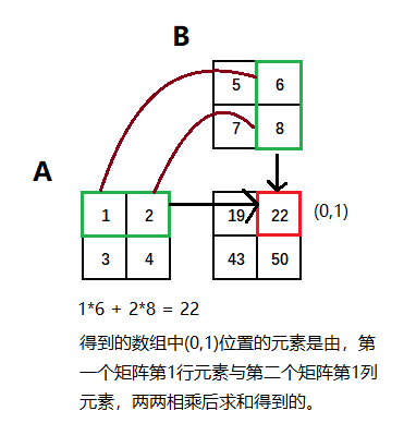
1 2 3 4 5 6 7 8 9 10 11 12 13 14 1 ,5 ).reshape(2 ,2 )1 , 2 ],3 , 4 ]])5 ,9 ).reshape(2 ,2 )5 , 6 ],7 , 8 ]])19 , 22 ],43 , 50 ]])
sigmoid()函数的用法及意义 [2] sigmoid函数也叫Logistic函数,用于隐层神经元输出,取值范围为(0,1),它可以将一个实数映射到(0,1)的区间,可以用来做二分类。
这就是sigmoid函数的表达式,这个函数在伯努利分布上非常好用,现在看看他的图像就清楚
可以看到在趋于正无穷或负无穷时,函数趋近平滑状态,sigmoid函数因为输出范围(0,1),所以二分类的概率常常用这个函数,事实上logistic回归采用这个函数很多教程也说了以下几个优点
1 值域在0和1之间
2 函数具有非常好的对称性
函数对输入超过一定范围就会不敏感sigmoid的输出在0和1之间,我们在二分类任务中,采用sigmoid的输出的是事件概率,也就是当输出满足满足某一概率条件我们将其划分正类,不同于svm。
代码:
1 2 3 4 5 6 7 8 9 10 11 12 13 14 15 16 17 18 19 20 from matplotlib import pyplot as pltimport numpy as npimport mathdef sigmoid_function (z ):for num in z:1 /(1 + math.exp(-num)))return fzif __name__ == '__main__' :10 , 10 , 0.01 )'Sigmoid Function' )'z' )'σ(z)' )
输出函数图像:
Numpy中的shape函数的用法详解 [3] 摘要 x.shape[0] will give the number of rows in an array. In your case it will give output 10. If you will type x.shape[1], it will print out the number of columns i.e 1024.
详解 中文解释 shape函数的功能是读取矩阵的长度,比如shape[0]就是读取矩阵第一维度的长度,相当于行数。它的输入参数可以是一个整数表示维度,也可以是一个矩阵。shape函数返回的是一个元组,表示数组(矩阵)的维度,例子如下:
数组(矩阵)只有一个维度时,shape只有shape[0],返回的是该一维数组(矩阵)中元素的个数,通俗点说就是返回列数,因为一维数组只有一行,一维情况中array创建的可以看做list(或一维数组)
示例代码:
1 2 3 4 5 6 7 8 9 10 11 12 >>> a=np.array([1 ,2 ])>>> a1 , 2 ])>>> a.shape2L ,)>>> a.shape[0 ]2L >>> a.shape[1 ]"<pyshell#63>" , line 1 , in <module>1 ]tuple index out of range
数组有两个维度(即行和列)时,和我们的逻辑思维一样,a.shape返回的元组表示该数组的行数与列数,请看下例:
示例代码:
1 2 3 4 5 6 7 8 9 10 11 12 >>> a=np.array([[1 ,2 ],[3 ,4 ]]) >>> a1 , 2 ],3 , 4 ]])>>> a.shape2L , 2L )>>> b=np.array([[1 ,2 ,3 ],[4 ,5 ,6 ]])>>> b1 , 2 , 3 ],4 , 5 , 6 ]])>>> b.shape2L , 3L )
英文解释 x[0].shape will give the Length of 1st row of an array. x.shape[0] will give the number of rows in an array. In your case it will give output 10. If you will type x.shape[1], it will print out the number of columns i.e 1024. If you would type x.shape[2], it will give an error, since we are working on a 2-d array and we are out of index. Let me explain you all the uses of ‘shape’ with a simple example by taking a 2-d array of zeros of dimension 3x4.
示例代码:
1 2 3 4 5 6 7 8 9 10 11 12 13 14 15 16 17 18 19 20 21 22 23 24 25 26 27 28 29 30 31 32 33 34 35 36 37 38 39 40 41 42 43 44 45 import numpy as np3 ,4 ))0. 0. 0. 0. ]0. 0. 0. 0. ]0. 0. 0. 0. ]]0 ]0. , 0. , 0. , 0. ])0 ].shape4 ,)1 ].shape4 ,)3 , 4 )0 ]3 1 ]3 1 ]4 range 2 ]input -20 -4b202d084bc7> in <module>()tuple index out of range
NumPy 切片和索引 [4] ndarray对象的内容可以通过索引或切片来访问和修改,与 Python 中 list 的切片操作一样。
ndarray 数组可以基于 0 - n 的下标进行索引,切片对象可以通过内置的 slice 函数,并设置 start, stop 及 step 参数进行,从原数组中切割出一个新数组。
实例:
1 2 3 4 5 6 7 8 9 import numpy as np 10 ) slice (2 ,7 ,2 ) print (a[s])
输出结果为:
冒号 : 的解释:如果只放置一个参数,如 **[2]**,将返回与该索引相对应的单个元素。如果为 **[2:]**,表示从该索引开始以后的所有项都将被提取。如果使用了两个参数,如 **[2:7]**,那么则提取两个索引(不包括停止索引)之间的项。
多维数组同样适用上述索引提取方法:
1 2 3 4 5 6 7 8 9 import numpy as np1 ,2 ,3 ],3 ,4 ,5 ],4 ,5 ,6 ]])'从数组索引 a[1:] 处开始切割' )1 :])
输出结果为:
1 2 3 4 5 6 [[1 2 3] [3 4 5] [4 5 6]] 1 :] 处开始切割[[3 4 5] [4 5 6]]
批量梯度下降[5] 批量梯度下降法 批量梯度下降法 是最原始的形式,它是指在每一次迭代时 使用所有样本 来进行梯度的更新。
随机梯度下降法 随机梯度下降法 不同于批量梯度下降,随机梯度下降是在每次迭代时 使用一个样本 来对参数进行更新(mini-batch size =1)。
小批量梯度下降法 什么是小批量梯度下降? 具体的说:在算法的每一步,我们从具有 训练集(已经打乱样本的顺序) 中随机抽出 一小批量(mini-batch)样本
参考文献 :
[1] 越来越胖的GuanRunwei.简述Sigmoid函数(附Python代码)[G/OL].CSDN,2019(2019-11-25).https://blog.csdn.net/qq_38890412/article/details/103246057
[2] 付修磊.Numpy中的shape函数的用法详解[G/OL].CSDN,2018(2018-01-17).https://blog.csdn.net/qq_38669138/article/details/79084275
[3] Animesh Johri.x.shape[0] vs x[0].shape in NumPy[G/OL].stackoverflow,2018(2018-9-22).https://stackoverflow.com/questions/48134598/x-shape0-vs-x0-shape-in-numpy
[4] RUNOOB.COM编者.NumPy 切片和索引[G/OL].RUNOOB.COM,2021..https://www.runoob.com/numpy/numpy-indexing-and-slicing.html
[5] G-kdom.批量梯度下降(BGD)、随机梯度下降(SGD)、小批量梯度下降(MBGD)[G/OL].知乎,2019(2019-7-12).https://zhuanlan.zhihu.com/p/72929546